3 Vacuum Expectation Values and Two-Point Functions
3.1 Motivation
The discretized path integral can be calculated numerically. In lattice QCD, one has access to path-integral expectation values, but not to the Hamiltonian directly. This raises a fundamental question:
Problem. Assuming that we know only thermal expectation values of time-ordered products of field operators, how do we extract the energy levels of the theory?
The answer proceeds in two steps:
- The \(T \to \infty\) limit of thermal expectation values gives vacuum expectation values.
- Energy levels can be extracted from the time-dependence of two-point functions.
3.2 The Effective Hamiltonian
Recall that the transfer matrix \[ \hat{T}(\tau) = e^{-\frac{\tau}{2}\hat{V}}\,e^{-\tau\hat{K}}\,e^{-\frac{\tau}{2}\hat{V}} = e^{-\tau\hat{H} + O(\tau^2)} \] approximates the Euclidean evolution operator for a single time step. It is convenient to define the effective Hamiltonian \[ \hat{H}_{\mathrm{eff}}(\tau) \stackrel{\mathrm{def}}{=} -\frac{1}{\tau}\log\hat{T}(\tau). \] By construction, \(\hat{H}_{\mathrm{eff}}(\tau)\) depends on \(\tau\) while \(\hat{H}\) does not, and \[ \lim_{\tau\to 0}\hat{H}_{\mathrm{eff}}(\tau) = \hat{H}. \] The ground state of \(\hat{H}\) is the vacuum \(|\Omega\rangle\). The ground state of \(\hat{H}_{\mathrm{eff}}(\tau)\) is denoted \(|\Omega_{\mathrm{eff}}\rangle\): it is an approximation of \(|\Omega\rangle\), with \[ \lim_{\tau\to 0}|\Omega_{\mathrm{eff}}(\tau)\rangle = |\Omega\rangle. \] In the following we drop the subscript “eff” for brevity, writing \(|\Omega\rangle\) and \(E_n\) for both the exact and discretized quantities.
3.3 \(T \to \infty\) Limit and Vacuum Expectation Values
Assume for simplicity that the spectrum of \(\hat{H}\) is discrete (this is not essential). Label the energy eigenstates in non-decreasing order: \[ \hat{H}|E_n\rangle = E_n|E_n\rangle, \qquad E_0 < E_1 \leq E_2 \leq \cdots, \qquad |E_0\rangle \equiv |\Omega\rangle. \]
The partition function and thermal expectation value are \[ Z = \mathrm{tr}\,e^{-T\hat{H}} = \sum_{n=0}^\infty e^{-TE_n}, \] \[ \frac{1}{Z}\mathrm{tr}\!\left\{e^{-T\hat{H}}\hat{A}\right\} = \frac{\displaystyle\sum_n e^{-TE_n}\langle E_n|\hat{A}|E_n\rangle}{\displaystyle\sum_n e^{-TE_n}}. \]
As \(T\to\infty\), the lowest eigenvalue \(E_0\) dominates because \(e^{-TE_0} \gg e^{-TE_n}\) for all \(n \neq 0\). Therefore \[ \lim_{T\to\infty}\frac{1}{Z}\mathrm{tr}\!\left\{e^{-T\hat{H}}\hat{A}\right\} = \frac{e^{-TE_0}\langle E_0|\hat{A}|E_0\rangle}{e^{-TE_0}} = \langle\Omega|\hat{A}|\Omega\rangle. \]
The same argument applies in the discrete-time formulation with \(\hat{T}^{T/\tau}\) and \(\hat{H}_{\mathrm{eff}}\) in place of \(e^{-T\hat{H}}\) and \(\hat{H}\): \[ \lim_{T\to\infty}\frac{1}{Z}\mathrm{tr}\!\left\{\hat{T}^{T/\tau}\hat{A}\right\} = \langle\Omega|\hat{A}|\Omega\rangle. \]
3.4 Spectral Decomposition of the Vacuum 2pt Function
Define the thermal two-point function for \(t > 0\), \[ C_T(t) \stackrel{\mathrm{def}}{=} \frac{1}{Z}\mathrm{tr}\!\left\{e^{-T\hat{H}}\hat{A}(t)\hat{B}(0)\right\} = \langle A(t)B(0)\rangle_{\text{p.b.c. in time}}, \] where \(\hat{A}(t) = e^{t\hat{H}}\hat{A}\,e^{-t\hat{H}}\) is the Euclidean–Heisenberg picture operator. Its \(T\to\infty\) limit defines the vacuum 2pt function \[ C_\infty(t) \equiv \lim_{T\to\infty} C_T(t). \]
We derive its spectral decomposition in four steps.
Step ① — Apply the \(T\to\infty\) result of the previous section: \[ C_\infty(t) = \langle\Omega|\hat{A}(t)\hat{B}(0)|\Omega\rangle. \]
Step ② — Expand using the definition of \(\hat{A}(t)\): \[ = \langle\Omega|e^{t\hat{H}}\hat{A}\,e^{-t\hat{H}}\hat{B}|\Omega\rangle. \]
Step ③ — Use \(\hat{H}|\Omega\rangle = E_0|\Omega\rangle\) to pull out the vacuum energy: \[ = \langle\Omega|\hat{A}\,e^{-t(\hat{H}-E_0)}\hat{B}|\Omega\rangle. \]
Step ④ — Insert the completeness relation \(\mathbf{1} = \sum_{n=0}^\infty |E_n\rangle\langle E_n|\): \[ C_\infty(t) = \sum_{n=0}^\infty e^{-t(E_n-E_0)}\underbrace{\langle\Omega|\hat{A}|E_n\rangle\langle E_n|\hat{B}|\Omega\rangle}_{C_n}. \]
This is the spectral decomposition of the vacuum 2pt function. Separating the \(n=0\) term, \[ C_\infty(t) = \langle\Omega|\hat{A}|\Omega\rangle\langle\Omega|\hat{B}|\Omega\rangle + \sum_{n=1}^\infty C_n\,e^{-t(E_n-E_0)}, \] where \(C_n = \langle\Omega|\hat{A}|E_n\rangle\langle E_n|\hat{B}|\Omega\rangle\) and the \(n=0\) term is recognized as \(\lim_{T\to\infty}\langle A\rangle\langle B\rangle\).
Note that energies are always defined up to an arbitrary additive constant — only energy differences \(E_n - E_0\) have physical meaning.
3.5 Connected Two-Point Function and Energy Levels
The constant term \(\langle\Omega|\hat{A}|\Omega\rangle\langle\Omega|\hat{B}|\Omega\rangle\) carries no information about energy levels. Subtracting it defines the connected two-point function (also called correlator): \[ C_T^{\mathrm{conn}}(t) \stackrel{\mathrm{def}}{=} \langle A(t)B(0)\rangle - \langle A\rangle\langle B\rangle. \]
Taking \(T\to\infty\), \[ C_\infty^{\mathrm{conn}}(t) \equiv \lim_{T\to\infty} C_T^{\mathrm{conn}}(t) = \sum_{n=1}^\infty C_n\,e^{-t(E_n-E_0)}. \]
The low-lying energy levels can be extracted from the large-\(t\) behaviour: \[ C_\infty^{\mathrm{conn}}(t) \xrightarrow{t \gg 0} C_1\,e^{-t(E_1-E_0)} + C_2\,e^{-t(E_2-E_0)} + O\!\left(e^{-t(E_3-E_0)}\right). \]
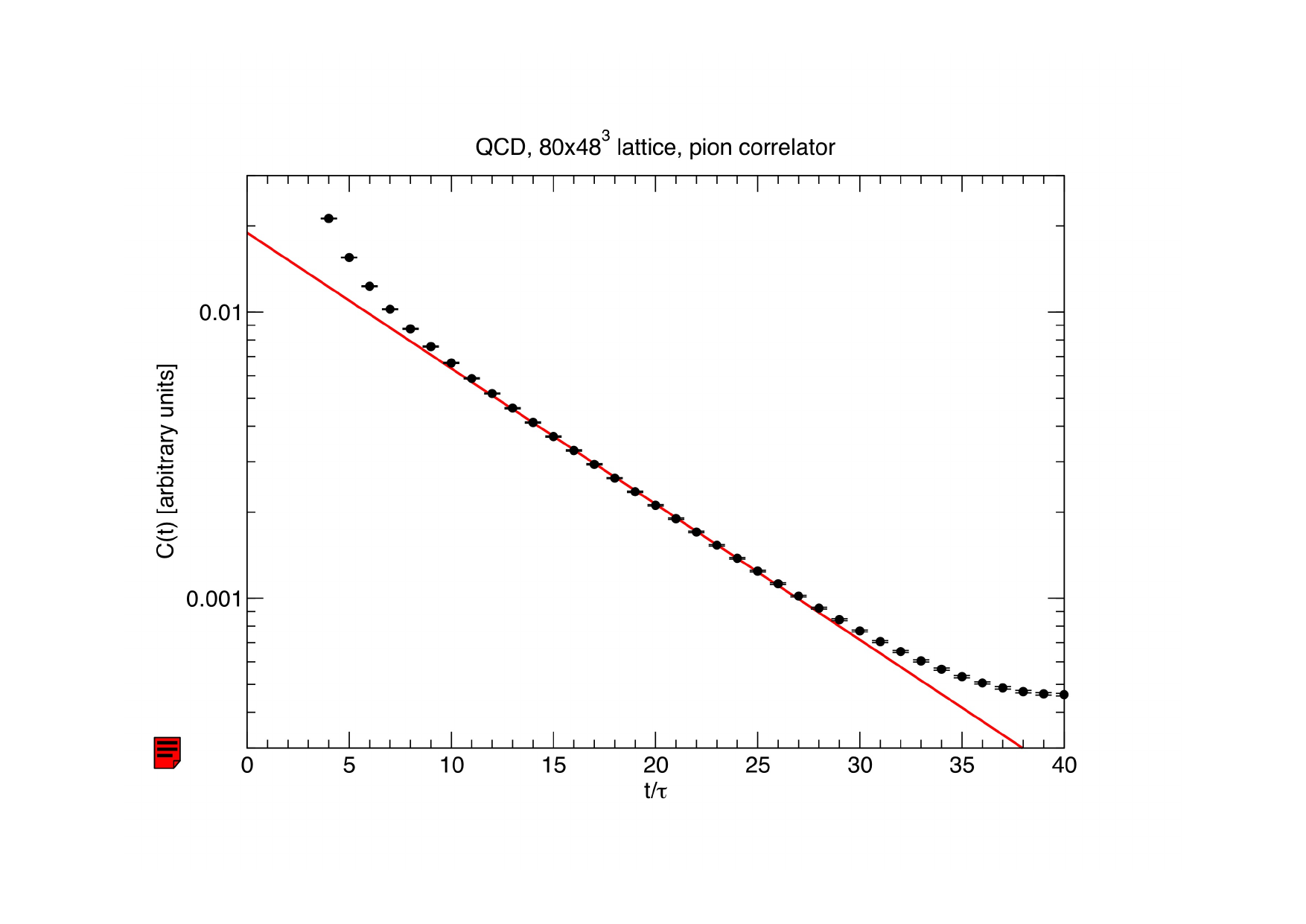
At sufficiently large \(t\) the correlator is dominated by the single exponential \(C_1 e^{-t(E_1-E_0)}\), from which the gap \(E_1-E_0\) can be read off directly as the slope on a logarithmic scale. This is how energy levels are extracted in practice in lattice simulations.
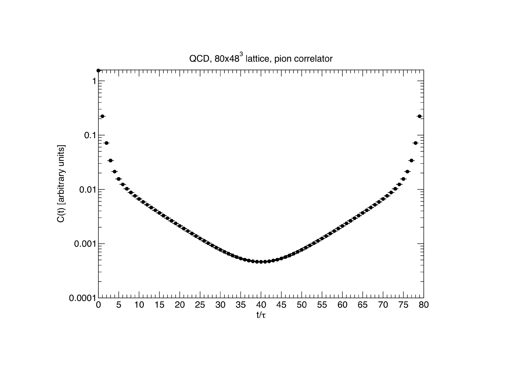
3.6 Example: Pion Correlator in Lattice QCD
The figures below show a pion correlator computed in QCD on an \(80\times48^3\) lattice.
3.7 Energy Levels as Poles of the Two-Point Function
Specialize to the case \(\hat{B} = \hat{A}\) and extend the definition of the vacuum 2pt function to all real \(t\) via time-ordering: \[ C_\infty(t) = \langle\Omega|\,\mathcal{T}\,\hat{A}(t)\hat{A}(0)\,|\Omega\rangle = \lim_{T\to\infty}\langle\mathcal{T}\,A(t)A(0)\rangle. \] Repeating the four-step derivation of the spectral decomposition for both signs of \(t\), \[ C_\infty(t) = \begin{cases} \langle\Omega|\hat{A}(t)\hat{A}(0)|\Omega\rangle = \langle\Omega|\hat{A}\,e^{-t(\hat{H}-E_0)}\hat{A}|\Omega\rangle, & t>0,\\[4pt] \langle\Omega|\hat{A}(0)\hat{A}(t)|\Omega\rangle = \langle\Omega|\hat{A}\,e^{+t(\hat{H}-E_0)}\hat{A}|\Omega\rangle, & t<0. \end{cases} \] Inserting completeness yields the spectral decomposition for arbitrary \(t\): \[ C_\infty(t) = \sum_{n=0}^\infty c_n\,e^{-|t|(E_n-E_0)} = \big(\langle\Omega|\hat{A}|\Omega\rangle\big)^2 + \sum_{n=1}^\infty c_n\,e^{-|t|(E_n-E_0)}, \] with \(c_n = \langle\Omega|\hat{A}|E_n\rangle\langle E_n|\hat{A}|\Omega\rangle = |\langle\Omega|\hat{A}|E_n\rangle|^2 \geq 0\). The connected 2pt function is then \[ C_\infty^{\mathrm{conn}}(t) = \sum_{n=1}^\infty c_n\,e^{-|t|\,\Delta E_n}, \qquad \Delta E_n \equiv E_n - E_0. \]
We now look at its Fourier transform, which exposes the energy levels as poles.
3.7.1 Continuous time
Assume a discrete spectrum (valid in finite volume): \[ \widetilde{C}_\infty^{\mathrm{conn}}(p_0) = \int_{-\infty}^{\infty} dt\,e^{ip_0 t}\,C_\infty^{\mathrm{conn}}(t). \] Using \[ \int_{-\infty}^{\infty} dt\,e^{ip_0 t}\,e^{-|t|\omega} = \left.\frac{e^{ip_0 t - t\omega}}{ip_0 - \omega}\right|_{0}^{\infty} + \left.\frac{e^{ip_0 t + t\omega}}{ip_0 + \omega}\right|_{-\infty}^{0} = \frac{1}{\omega - ip_0} + \frac{1}{\omega + ip_0} = \frac{2\omega}{p_0^2 + \omega^2}, \] we obtain \[ \widetilde{C}_\infty^{\mathrm{conn}}(p_0) = \sum_{n=1}^\infty \frac{2 c_n\,\Delta E_n}{p_0^2 + (E_n-E_0)^2}. \] This is analytically continued to \(p_0 \in \mathbb{C}\) except for simple poles at \[ p_0 = \pm i\,\Delta E_n. \]
3.7.2 Discrete time
In discrete time, the Fourier transform is a sum, \[ \widetilde{C}_\infty^{\mathrm{conn}}(p_0) = \sum_{t\in\tau\mathbb{Z}} e^{ip_0 t}\,C_\infty^{\mathrm{conn}}(t), \] and the geometric series gives \[ \sum_{t\in\tau\mathbb{Z}} e^{ip_0 t}\,e^{-|t|\omega} = \sum_{k=0}^\infty e^{(ip_0-\omega)\tau k} + \sum_{k=0}^\infty e^{(-ip_0-\omega)\tau k} - 1 = \frac{1}{1 - e^{(ip_0-\omega)\tau}} + \frac{1}{1 - e^{(-ip_0-\omega)\tau}} - 1, \] so that \[ \widetilde{C}_\infty^{\mathrm{conn}}(p_0) = \sum_{n=1}^\infty c_n\left\{\frac{1}{1 - e^{(ip_0-\Delta E_n)\tau}} + \frac{1}{1 - e^{(-ip_0-\Delta E_n)\tau}} - 1\right\}. \] This function is periodic in \(p_0\) with period \(2\pi/\tau\), \[ \widetilde{C}_\infty^{\mathrm{conn}}\!\left(p_0 + \tfrac{2\pi}{\tau}\right) = \widetilde{C}_\infty^{\mathrm{conn}}(p_0), \] and analytic except for simple poles at \[ e^{(ip_0 - \Delta E_n)\tau} = 1 \quad\Longleftrightarrow\quad p_0 = \pm i\,\Delta E_n + \frac{2\pi}{\tau}\,k, \qquad k \in \mathbb{Z}. \]
In both cases, the energy differences \(\Delta E_n\) are read off from the poles of the Fourier-transformed 2pt function. This pole structure is exact only at finite volume; in the infinite-volume limit one generally has both poles (stable single-particle states) and cuts (multi-particle thresholds).
3.8 The Simplest 2pt Function: Free Scalar Theory
We now compute \(\langle\varphi(x)\varphi(y)\rangle\) explicitly in the free scalar theory on a finite lattice. Periodic boundary conditions are imposed in space and time: \[ S = \sum_x \tau a^3\left\{\tfrac{1}{2}\big(\partial_\mu^f \varphi\big)^2 + \tfrac{m^2}{2}\,\varphi^2\right\}, \] with \[ x_0 = 0,\tau,\ldots,T-\tau, \qquad x_k = 0, a, \ldots, L-a \quad (k=1,2,3), \] \[ \varphi(x_0+T,\mathbf{x}) = \varphi(x_0,\mathbf{x}), \qquad \varphi(x_0,\mathbf{x}+L\mathbf{e}_k) = \varphi(x_0,\mathbf{x}), \] and the forward derivatives \[ \partial_0^f\varphi(x_0,\mathbf{x}) = \frac{\varphi(x_0+\tau,\mathbf{x})-\varphi(x_0,\mathbf{x})}{\tau}, \qquad \partial_k^f\varphi(x_0,\mathbf{x}) = \frac{\varphi(x_0,\mathbf{x}+a\mathbf{e}_k)-\varphi(x_0,\mathbf{x})}{a}. \] We want to calculate the lattice propagator \[ \langle\varphi(x)\varphi(y)\rangle = \frac{\int [d\varphi]\,e^{-S}\,\varphi(x)\varphi(y)}{\int [d\varphi]\,e^{-S}}. \]
The strategy is to recast the action as a quadratic form \(S = \tfrac{1}{2}(\varphi, A\varphi)\) for some real, symmetric, positive-definite operator \(A\), then use the Gaussian-integration result \(\langle\varphi(x)\varphi(y)\rangle = (A^{-1})_{xy}\), then diagonalize \(A\) with plane waves.
3.8.1 Step 1 — Scalar product
Define a scalar product on the space of lattice fields: \[ (\varphi_1,\varphi_2) \stackrel{\mathrm{def}}{=} \sum_x \tau a^3\,\varphi_1(x)\,\varphi_2(x). \]
3.8.2 Step 2 — Transposition of derivatives
We claim that \(\big(\partial_\mu^f\big)^T = -\partial_\mu^b\), where the backward derivatives are \[ \partial_0^b\varphi(x_0,\mathbf{x}) = \frac{\varphi(x_0,\mathbf{x})-\varphi(x_0-\tau,\mathbf{x})}{\tau}, \qquad \partial_k^b\varphi(x) = \frac{\varphi(x_0,\mathbf{x})-\varphi(x_0,\mathbf{x}-a\mathbf{e}_k)}{a}. \] Proof for \(\mu=0\) (the spatial cases are identical): \[ \big(\varphi_2,(\partial_0^f)^T\varphi_1\big) \stackrel{\text{①}}{=} \big(\partial_0^f\varphi_2,\varphi_1\big) \stackrel{\text{②}}{=} \sum_x \tau a^3\,\frac{\varphi_2(x_0+\tau,\mathbf{x}) - \varphi_2(x_0,\mathbf{x})}{\tau}\,\varphi_1(x). \] Splitting and using periodicity in time (step ③: shift \(x_0 \to x_0 - \tau\) in the first sum), \[ = \sum_x a^3\,\varphi_2(x_0,\mathbf{x})\,\varphi_1(x_0-\tau,\mathbf{x}) - \sum_x a^3\,\varphi_2(x)\,\varphi_1(x) = \sum_x \tau a^3\,\varphi_2(x)\,\frac{-\varphi_1(x) + \varphi_1(x_0-\tau,\mathbf{x})}{\tau} = \big(\varphi_2,-\partial_0^b\varphi_1\big). \] Since this holds for all \(\varphi_1,\varphi_2\), \((\partial_0^f)^T = -\partial_0^b\). The same argument with the spatial periodicity gives \((\partial_k^f)^T = -\partial_k^b\).
3.8.3 Step 3 — Action as a quadratic form
Using the bilinearity of the scalar product and \((\partial_\mu^f)^T = -\partial_\mu^b\): \[ S = \tfrac{1}{2}\sum_\mu (\partial_\mu^f\varphi,\partial_\mu^f\varphi) + \tfrac{m^2}{2}(\varphi,\varphi) \stackrel{\text{①}}{=} -\tfrac{1}{2}\sum_\mu (\varphi,\partial_\mu^b\partial_\mu^f\varphi) + \tfrac{m^2}{2}(\varphi,\varphi) \stackrel{\text{②}}{=} \tfrac{1}{2}\big(\varphi,A\varphi\big), \] with \[ A \equiv -\sum_\mu \partial_\mu^b \partial_\mu^f + m^2. \] Exercise: \(A\) is real, symmetric, and strictly positive-definite.
3.8.4 Step 4 — Gaussian integration
With \(S = \tfrac{1}{2}(\varphi,A\varphi) = \tfrac{1}{2}\sum_{x,y}\tau a^3\,\varphi(x)\,\big[\tau a^3 A_{xy}\big]\,\varphi(y)\) — note the \(\tau a^3\) factor in the scalar product — the Gaussian integral gives \[ \langle\varphi(x)\varphi(y)\rangle = \frac{\int [d\varphi]\,\varphi(x)\varphi(y)\,e^{-\tfrac{1}{2}(\varphi,A\varphi)}}{\int [d\varphi]\,e^{-\tfrac{1}{2}(\varphi,A\varphi)}} = \big(A^{-1}\big)_{xy}. \] This can be derived by integration by parts: \[ 0 = \int [d\varphi]\,\frac{\partial}{\partial\varphi(x)}\!\left\{\varphi(y)\,e^{-\tfrac{1}{2}(\varphi,A\varphi)}\right\} = \int [d\varphi]\left\{\delta_{xy} - \varphi(y)\,(A\varphi)(x)\right\}e^{-S}, \] which after dividing by the partition function gives \(\sum_z A_{xz}\langle\varphi(z)\varphi(y)\rangle = \delta_{xy}\), i.e. \(\langle\varphi(x)\varphi(y)\rangle = (A^{-1})_{xy}\).
3.8.5 Step 5 — Diagonalizing \(A\) with plane waves
In the continuum, \(A \propto -\partial^2 + m^2\) is diagonalized by plane waves \(e^{ipx}\). The same is true on the lattice. Define \[ v_p(x) = e^{ipx}. \] The periodic boundary conditions in time and space quantize the momenta: \[ e^{ip_0(x_0+T)+i\mathbf{p}\cdot\mathbf{x}} = e^{ipx} \;\Longleftrightarrow\; e^{ip_0 T} = 1 \;\Longleftrightarrow\; p_0 \in \tfrac{2\pi}{T}\mathbb{Z}, \] \[ e^{ip_0 x_0 + i\mathbf{p}\cdot(\mathbf{x}+L\mathbf{e}_k)} = e^{ipx} \;\Longleftrightarrow\; e^{ip_k L} = 1 \;\Longleftrightarrow\; p_k \in \tfrac{2\pi}{L}\mathbb{Z}. \] The lattice spacings further introduce a redundancy: shifts of \(p_0\) by \(2\pi/\tau\) or of \(p_k\) by \(2\pi/a\) leave \(v_p(x)\) unchanged at every lattice point, because \(x_0/\tau \in \mathbb{Z}\) and \(x_k/a \in \mathbb{Z}\): \[ v_{p_0+2\pi/\tau,\,\mathbf{p}}(x) = e^{ipx}\,e^{i 2\pi x_0/\tau} = v_p(x), \qquad v_{p,\,\mathbf{p}+(2\pi/a)\mathbf{e}_k}(x) = e^{ipx}\,e^{i 2\pi x_k/a} = v_p(x). \] Each plane wave is therefore taken exactly once by restricting \(p\) to a Brillouin zone: \[ \Pi = \left\{p \in \tfrac{2\pi}{T}\mathbb{Z}\times\tfrac{2\pi}{L}\mathbb{Z}^3 \;\middle|\; 0 \leq p_0 < \tfrac{2\pi}{\tau},\; 0 \leq p_k < \tfrac{2\pi}{a}\right\}, \] or equivalently, centered around the origin, \[ \Pi = \left\{p \in \tfrac{2\pi}{T}\mathbb{Z}\times\tfrac{2\pi}{L}\mathbb{Z}^3 \;\middle|\; -\tfrac{\pi}{\tau} < p_0 \leq \tfrac{\pi}{\tau},\; -\tfrac{\pi}{a} < p_k \leq \tfrac{\pi}{a}\right\}. \] The lattice momenta thus form a finite set of \((T/\tau)\times(L/a)^3\) values — the same as the number of lattice points, as required.