1 Quantum Mechanics of Lattice Discretized Scalar Field Theory
1.1 Roadmap
There are two standard routes from classical field theory to lattice QFT.
The standard textbook route proceeds as follows. Starting from a classical field theory with action \(S(\varphi)\), one quantizes via the path integral, \[ \langle A \rangle = \frac{1}{Z} \int \mathcal{D}\varphi \, e^{iS(\varphi)} A(\varphi), \] applies a Wick rotation to obtain Euclidean QFT, \[ \langle A \rangle = \frac{1}{Z} \int \mathcal{D}\varphi \, e^{-S_E(\varphi)} A(\varphi), \] and then discretizes on a 4d lattice to arrive at lattice QFT.
The route followed in this course is Hamiltonian-based. Starting again from the classical action, one passes to the Hamiltonian formalism via a Legendre transform, canonically quantizes to obtain the Hamiltonian formalism for QFT, discretizes space on a 3d lattice, and then performs a Wick rotation followed by a time-discretized path integral to arrive at lattice QFT. This route makes the physical content more transparent at each step.
1.2 Classical \(\varphi^4\) Theory: Action Formalism
Let \(\varphi : \mathbb{R}^4 \to \mathbb{R}\), \(x \mapsto \varphi(x)\), be a real scalar field. The Lagrangian density is \[ \mathcal{L}(\varphi(x), \partial\varphi(x), \ldots) = \frac{1}{2}\,\partial_\mu\varphi\,\partial^\mu\varphi(x) - \frac{m^2}{2}\,\varphi^2(x) - \frac{1}{4!}\,\varphi^4(x), \] where \(g = \mathrm{diag}(+1,-1,-1,-1)\). The action on a domain \(V \subset \mathbb{R}^4\) is \[ S_V(\varphi) = \int_V d^4x\;\mathcal{L}(\varphi(x), \partial\varphi(x), \ldots). \]
The field \(\varphi\) satisfies the equations of motion if and only if \[ \frac{\delta S_V}{\delta \varphi(x)} = 0 \quad \text{for every } x \in \mathrm{int}(V), \] which is equivalent to requiring \(S_V(\varphi + \eta) = S_V(\varphi) + O(\eta^2)\) for every \(\eta\) with compact support in the interior of \(V\).
To derive the equations of motion explicitly, expand \[ S_V(\varphi+\eta) = S_V(\varphi) + \int_V d^4x \left[\partial_\mu\varphi\,\partial^\mu\eta - m^2\varphi\eta - \frac{1}{3!}\varphi^3\eta\right](x) + O(\eta^2). \] Integrating by parts and using \(\eta|_{\partial V} = 0\), \[ S_V(\varphi+\eta) = S_V(\varphi) + \int_{\partial V} dS^\mu\,\eta\,\partial_\mu\varphi - \int_V d^4x\;\eta(x)\left[\partial_\mu\partial^\mu\varphi + m^2\varphi + \frac{1}{3!}\varphi^3\right](x) + O(\eta^2). \] The boundary term vanishes by hypothesis, so the condition \(S_V(\varphi+\eta)=S_V(\varphi)+O(\eta^2)\) for all such \(\eta\) yields the equations of motion \[ \partial_\mu\partial^\mu\varphi + m^2\varphi + \frac{1}{3!}\varphi^3 = 0. \]
1.3 Classical \(\varphi^4\) Theory: Hamiltonian Formalism
In the Hamiltonian formalism, time and space are treated differently. Write \(\varphi_t(\mathbf{x}) = \varphi(t,\mathbf{x})\) and \(\dot{\varphi}_t(\mathbf{x}) = \frac{\partial}{\partial t}\varphi(t,\mathbf{x})\). The Lagrangian is \[ L(\varphi_t, \dot{\varphi}_t) = \int d^3x\;\mathcal{L}(\varphi(t,\mathbf{x}), \partial\varphi(t,\mathbf{x})) = \int d^3x\left[\frac{1}{2}\dot{\varphi}_t^2 - \frac{1}{2}\sum_{k=1}^3 \partial_k\varphi_t\,\partial_k\varphi_t - \frac{m^2}{2}\varphi_t^2 - \frac{1}{4!}\varphi_t^4\right](\mathbf{x}), \] which can be written as \(L(\varphi_t,\dot{\varphi}_t) = \int d^3x\,\tfrac{1}{2}\dot{\varphi}_t^2 - V(\varphi_t)\).
The canonical momentum associated to \(\varphi_t\) is \[ \pi_t(\mathbf{x}) = \frac{\delta L}{\delta \dot{\varphi}_t(\mathbf{x})} = \dot{\varphi}_t(\mathbf{x}). \]
The Hamiltonian is the Legendre transform of the Lagrangian: \[ H(\pi_t, \varphi_t) = \int d^3x\;\pi_t(\mathbf{x})\dot{\varphi}_t(\mathbf{x}) - L(\varphi_t, \dot{\varphi}_t) = \int d^3x\;\frac{1}{2}\pi_t^2(\mathbf{x}) + V(\varphi_t), \] \[ H(\pi_t, \varphi_t) = \int d^3x \left[\frac{1}{2}\pi_t^2 + \frac{1}{2}(\nabla\varphi_t)^2 + \frac{m^2}{2}\varphi_t^2 + \frac{1}{4!}\varphi_t^4\right](\mathbf{x}). \]
The equations of motion are equivalent to the Hamilton equations: \[ \dot{\varphi}_t = \frac{\delta H}{\delta \pi_t} = \pi_t, \qquad \dot{\pi}_t = -\frac{\delta H}{\delta \varphi_t} = \nabla^2\varphi_t - m^2\varphi_t - \frac{1}{3!}\varphi_t^3. \]
1.4 Canonical Quantization
Canonical quantization proceeds in four steps.
Step 1. Upgrade \(\varphi(\mathbf{x})\) and \(\pi(\mathbf{x})\) to operators on some Hilbert space, satisfying the self-adjoint conditions (reflecting that the fields are real) \[ \varphi(\mathbf{x})^\dagger = \varphi(\mathbf{x}), \qquad \pi(\mathbf{x})^\dagger = \pi(\mathbf{x}), \] and the canonical commutation relations (CCR) \[ [\varphi(\mathbf{x}), \pi(\mathbf{y})] = i\delta^3(\mathbf{x}-\mathbf{y}), \qquad [\varphi(\mathbf{x}),\varphi(\mathbf{y})] = [\pi(\mathbf{x}),\pi(\mathbf{y})] = 0. \]
Step 2. The Hamiltonian is formally identical to the classical one: \[ H = \int d^3x \left[\frac{1}{2}\pi^2 + \frac{1}{2}(\nabla\varphi)^2 + \frac{m^2}{2}\varphi^2 + \frac{1}{4!}\varphi^4\right](\mathbf{x}). \]
Step 3. Time evolution follows the standard rules of quantum mechanics:
- Schrödinger picture: states evolve, \(|\psi(t)\rangle = e^{-iHt}|\psi(0)\rangle\); observables \(A\), \(\varphi(\mathbf{x})\), \(\pi(\mathbf{x})\), \(\ldots\) do not.
- Heisenberg picture: observables evolve, \(A(t) = e^{iHt} A e^{-iHt}\), with \(\varphi(t,\mathbf{x}) = e^{iHt}\varphi(\mathbf{x})e^{-iHt}\) and \(\pi(t,\mathbf{x}) = e^{iHt}\pi(\mathbf{x})e^{-iHt}\); states \(|\psi\rangle\) do not.
- Interaction picture: useful for perturbative expansions; not used in this course.
Step 4. The Hilbert space.
- For the free theory, the Hilbert space is the Fock space.
- In the general interacting case, the explicit construction of the Hilbert space is still an open problem. Physicists typically assume it exists and derive properties from general principles (axiomatic QFT).
A fundamental issue arises from the CCR: the right-hand side of \[ [\varphi(\mathbf{x}), \pi(\mathbf{y})] = i\delta^3(\mathbf{x}-\mathbf{y}) \times \mathbf{1} \] is not a genuine operator, since \(\delta^3(\mathbf{x}-\mathbf{y})\) is not a number for generic \(\mathbf{x},\mathbf{y}\) — in particular \(\delta^3(0) = \infty\). Two ways to handle this:
- Treat \(\varphi(\mathbf{x})\) and \(\pi(\mathbf{x})\) as distribution-valued operators.
- Regularize the theory. The regularization turns \(\varphi(\mathbf{x})\) and \(\pi(\mathbf{x})\) into honest operators. This is the approach followed in this course.
1.5 Lattice Regularization of Space
The regularization is implemented by replacing continuous 3d space with a lattice. There are two successive approximations:
| Continuous | Infinite lattice | Finite lattice | |
|---|---|---|---|
| Space | \(\mathbf{x} \in \mathbb{R}^3\) | \(\mathbf{x} \in a\mathbb{Z}^3\) | \(\mathbf{x} \in a\mathbb{I}_N^3\) |
| Coordinates | — | \(\mathbf{x}=(an_1,an_2,an_3),\; n_k\in\mathbb{Z}\) | \(\mathbf{x}=(an_1,an_2,an_3),\; n_k\in\mathbb{I}_N\) |
where \(a\) is the lattice spacing, \(\mathbb{I}_N = \{0,1,\ldots,N-1\}\), and \(|a\mathbb{I}_N^3| = N^3\) is the number of lattice points.
The dictionary between continuum and lattice objects is:
\[ \int d^3x\; f(\mathbf{x}) \;\longrightarrow\; \sum_{\mathbf{x}\in a\mathbb{I}_N^3} a^3 f(\mathbf{x}), \] \[ \delta^3(\mathbf{x}-\mathbf{y}) \;\longrightarrow\; a^{-3}\delta_{\mathbf{x},\mathbf{y}}, \] which satisfies the normalization \(\sum_{\mathbf{x}} a^3 \cdot a^{-3}\delta_{\mathbf{x},\mathbf{y}} = 1\).
The partial derivative \(\frac{\partial f}{\partial x_k}(\mathbf{x})\) is replaced by finite differences. The two natural choices are \[ \partial_k^f f(\mathbf{x}) = \frac{f(\mathbf{x}+a\mathbf{e}_k)-f(\mathbf{x})}{a} \quad \text{(forward derivative)}, \] \[ \partial_k^b f(\mathbf{x}) = \frac{f(\mathbf{x})-f(\mathbf{x}-a\mathbf{e}_k)}{a} \quad \text{(backward derivative)}. \] On the finite lattice, we impose periodic boundary conditions: the shifts \(\mathbf{x} \pm a\mathbf{e}_k\) are interpreted modulo \(aN\).
1.6 Scalar Field Theory on an \(N^3\) Lattice
After lattice regularization of space, the theory is defined by the following data.
Commutation relations. \[ [\hat{\varphi}(\mathbf{x}), \hat{\pi}(\mathbf{y})] = ia^{-3}\delta_{\mathbf{x},\mathbf{y}}, \qquad [\hat{\varphi}(\mathbf{x}),\hat{\varphi}(\mathbf{y})] = [\hat{\pi}(\mathbf{x}),\hat{\pi}(\mathbf{y})] = 0. \]
Hamiltonian. \[ H = \sum_{\mathbf{x}\in a\mathbb{I}_N^3} a^3 \left[\frac{1}{2}\hat{\pi}^2 + \frac{1}{2}\sum_{k=1}^3(\partial_k^f\hat{\varphi})^2 + \frac{m^2}{2}\hat{\varphi}^2 + \frac{1}{4!}\hat{\varphi}^4\right](\mathbf{x}). \]
Hilbert space. Let \(\mathcal{C}\) be the space of field configurations, \[ \mathcal{C} = \{\varphi : a\mathbb{I}_N^3 \to \mathbb{R}\} \cong \mathbb{R}^{N^3}. \] The Hilbert space is \[ \mathcal{H} = \left\{\psi : \mathcal{C} \to \mathbb{C} \;\Big|\; \int\!\left[\prod_{\mathbf{x}}d\varphi(\mathbf{x})\right]|\psi(\varphi)|^2 < +\infty\right\} \cong L^2(\mathbb{R}^{N^3}). \]
Equivalence with a point particle. Label the \(N^3\) lattice sites by an index \(\alpha = 0, 1, \ldots, N^3-1\) and set \[ \hat{q}_\alpha = \hat{\varphi}(\mathbf{x}), \qquad \hat{p}_\alpha = a^3\hat{\pi}(\mathbf{x}). \] Then \([\hat{q}_\alpha, \hat{p}_\beta] = i\delta_{\alpha\beta}\) and \([\hat{q}_\alpha,\hat{q}_\beta]=[\hat{p}_\alpha,\hat{p}_\beta]=0\): these are the position and momentum operators of a point particle in \(N^3\)-dimensional space. The Hamiltonian becomes \[ H = \sum_\alpha \frac{\hat{p}_\alpha^2}{2a^3} + V(\hat{q}), \] and the Hilbert space is \(L^2(\mathbb{R}^D)\) with \(D = N^3\).
Conclusion. Scalar field theory on an \(N^3\) lattice is mathematically equivalent to the quantum mechanics of a point particle in \(N^3\)-dimensional space.
1.7 Dirac Bra-Ket Notation
The simultaneous eigenstates of \(\hat{\varphi}(\mathbf{x})\) for all \(\mathbf{x}\) are denoted \(|\varphi\rangle\), where for each \(\mathbf{x}\) the eigenvalue \(\varphi(\mathbf{x})\) is a number: \[ \hat{\varphi}(\mathbf{x})|\varphi\rangle = \varphi(\mathbf{x})|\varphi\rangle. \] These states satisfy orthogonality and completeness relations, \[ \langle\varphi'|\varphi\rangle = \prod_{\mathbf{x}}\delta(\varphi'(\mathbf{x})-\varphi(\mathbf{x})), \qquad \int\!\left[\prod_{\mathbf{x}}d\varphi(\mathbf{x})\right]|\varphi\rangle\langle\varphi| = \mathbf{1}. \] The wave function of a state \(|\psi\rangle\) in the field basis is \(\psi(\varphi) = \langle\varphi|\psi\rangle\).
Similarly, the simultaneous eigenstates of \(\hat{\pi}(\mathbf{x})\) for all \(\mathbf{x}\) are denoted \(|\pi\rangle\): \[ \hat{\pi}(\mathbf{x})|\pi\rangle = \pi(\mathbf{x})|\pi\rangle, \] with orthogonality and completeness \[ \langle\pi'|\pi\rangle = \prod_{\mathbf{x}}2\pi\delta(\pi'(\mathbf{x})-\pi(\mathbf{x})), \qquad \int\!\left[\prod_{\mathbf{x}}\frac{d\pi(\mathbf{x})}{2\pi}\right]|\pi\rangle\langle\pi| = \mathbf{1}. \] The overlap between the two bases is \[ \langle\varphi|\pi\rangle = \exp\!\left\{i\sum_{\mathbf{x}}a^3\pi(\mathbf{x})\varphi(\mathbf{x})\right\}. \]
In the point-particle notation (\(\alpha\) indexing lattice sites): \[ \hat{q}_\alpha|q\rangle = q_\alpha|q\rangle, \quad \langle q'|q\rangle = \delta^D(q'-q), \quad \int d^Dq\,|q\rangle\langle q| = \mathbf{1}, \quad \psi(q)=\langle q|\psi\rangle, \] \[ \hat{p}_\alpha|p\rangle = p_\alpha|p\rangle, \quad \langle p'|p\rangle = (2\pi)^D\delta^D(p'-p), \quad \int\frac{d^Dp}{(2\pi)^D}|p\rangle\langle p| = \mathbf{1}, \quad \langle q|p\rangle = \exp\!\left\{i\sum_\alpha p_\alpha q_\alpha\right\}. \]
1.8 Euclidean QM and QFT
The Wick rotation replaces the Minkowski time evolution operator \(e^{-iHt}\) (\(t\) real) with the Euclidean one \(e^{-\tau H}\) (\(\tau\) real, \(\tau > 0\)), corresponding to \(t \to -i\tau\).
Why work in Euclidean time?
- Numerical simulations: efficient Monte Carlo algorithms exist only for Euclidean QFT, where the weight \(e^{-S_E}\) is real and positive.
- Theoretical control: when time is discretized, renormalization and the continuum limit are well understood only in the Euclidean framework.
Does this alter the physics? No, in the following senses:
- The Hilbert space, the Hamiltonian, the vacuum, and all operators in the Schrödinger picture are the same as in the Minkowskian formulation. The physics is the same; it is only encoded differently in time-dependent observables.
- The canonical ensemble density matrix \(\rho = \frac{1}{Z}e^{-\beta H}\) is the thermal state of the system in equilibrium. Here Euclidean time plays the role of \(\beta\), the inverse temperature. Euclidean QFT thus gives direct access to thermodynamic properties.
- Time-ordered Minkowskian and Euclidean \(n\)-point functions are related by analytic continuation (Wick rotation).
1.9 Wick Rotation and Euclidean Time
The analytic continuation from Minkowski to Euclidean time is justified by the following theorem (from the theory of analytic semigroups).
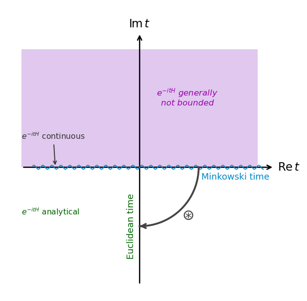
Theorem. Let \(H\) be a self-adjoint operator bounded from below, \(H \geq E_0\) for some \(E_0 \in \mathbb{R}\). Then:
The operator \(e^{-itH}\) is bounded, \(\|e^{-itH}\| < +\infty\), for every complex \(t\) with \(\mathrm{Im}\,t \leq 0\). In particular, for \(\mathrm{Im}\,t \leq 0\): \(e^{-itH}\) is defined on all of \(\mathcal{H}\) and is a continuous operator.
Note. For \(\tau > 0\): setting \(t = i\tau\) gives \(e^{-itH} = e^{\tau H}\), which diverges; setting \(t = -i\tau\) gives \(e^{-itH} = e^{-\tau H}\), which is well-defined. ✓
The function \(t \mapsto e^{-itH}\) is analytic for \(\mathrm{Im}\,t < 0\): it admits a convergent power series expansion around every such \(t\), with positive radius of convergence, converging in operator norm.
The function \(t \mapsto e^{-itH}\) is continuous (in operator norm) for \(\mathrm{Im}\,t \leq 0\).
The Wick rotation is the analytic continuation from positive Minkowski time (real \(t > 0\)) to Euclidean time \(\tau > 0\), along the contour \(t \to e^{-i\varphi}t\) with \(\varphi \in [0,\pi/2]\) in the lower half of the complex \(t\)-plane.
Example: time-ordered \(n\)-point functions (\(n=3\) for concreteness).
Let \(|\Omega\rangle\) be the ground state (vacuum) of \(H\). Assume time-ordering \(x_3^0 > x_2^0 > x_1^0\). The Minkowskian 3-point function is \[ C_M(x_1,x_2,x_3) = \langle\Omega|\hat{\varphi}_H(x_3)\hat{\varphi}_H(x_2)\hat{\varphi}_H(x_1)|\Omega\rangle, \] where \(\hat{\varphi}_H(x) = e^{iHx^0}\hat{\varphi}(\mathbf{x})e^{-iHx^0}\). Expanding, \[ C_M = e^{i(x_3^0-x_1^0)E_0}\langle\Omega|\hat{\varphi}(\mathbf{x}_3)\,e^{-i(x_3^0-x_2^0)H}\,\hat{\varphi}(\mathbf{x}_2)\,e^{-i(x_2^0-x_1^0)H}\,\hat{\varphi}(\mathbf{x}_1)|\Omega\rangle. \] The time differences \(x_3^0 - x_2^0 > 0\) and \(x_2^0 - x_1^0 > 0\) ensure convergence under the Wick rotation \(x_k^0 \to e^{-i\varphi}x_k^0\) with \(\varphi \in [0,\pi/2]\). At \(\varphi = \pi/2\) one obtains the Euclidean 3-point function \[ C_E(x_1,x_2,x_3) = \langle\Omega|\hat{\varphi}_E(x_3)\hat{\varphi}_E(x_2)\hat{\varphi}_E(x_1)|\Omega\rangle = e^{(x_3^0-x_1^0)E_0}\langle\Omega|\hat{\varphi}(\mathbf{x}_3)\,e^{-(x_3^0-x_2^0)H}\,\hat{\varphi}(\mathbf{x}_2)\,e^{-(x_2^0-x_1^0)H}\,\hat{\varphi}(\mathbf{x}_1)|\Omega\rangle, \] where \(x_k^0\) now denotes Euclidean time.